Machines and processes are controlled using many strategies, from simple ladder logic to custom algorithms for specialized process control, but proportional-integral-derivative (PID) is the most common control method. Different programmable logic controllers (PLCs) handle PID control loops in different ways. Some loops need to be set manually, while others can use an autotune process embedded in the PLC's software.

Even before loop tuning starts, the design may have created a slow-to-respond control loop with built-in lag. For example, a temperature sensor positioned a long distance from a heater can slow response to dynamic changes.

Changes in machines and processes due to disturbances and set point changes are why PID control is often needed. The amount, length of time, and rate of change of the process error are all part of the PID equation, as is correcting the error to bring the process variable closer to the set point. This blog post will look at the PID equation and some tuning tips, along with a brief review of autotuning and applications benefiting from PID control.

What is PID control?

The application almost always determines whether open- or closed-loop analog control is used. Many applications will work with on-off, closed-loop control using an analog sensor measuring temperature, pressure, level, or flow as an input to control a discrete output. The same analog sensors are also used for PID closed-loop control, but in a more complex strategy.

In on-off, closed-loop control of room temperature, for example, a heat or cooling cycle is triggered by hysteresis in the thermostat. When the room temperature is approximately 1°F or 2°F above the set point, a cooling cycle is turned on. Once the set point-or possibly 1°F or 2°F below the set point-is reached, the cooling cycle is turned off. This can result in a 2°-4°F swing in room temperature. The temperature swing can be even worse with a slight overshoot at the turn-off point and undershoot at the turn-on point. This temperature swing (error) around the set point is not accurate enough in many industrial control processes.

To reduce the process variable error, the closed-loop control function in PID controllers is commonly used. A PID controller reads a process variable (PV), compares it to a desired set point (SP) value, and uses a continuous feedback loop to adjust the control output.

The equation behind PID loops

For many control system programmers, PID loops can be difficult to set and tune. Many have forgotten the calculus involved or never learned it, but a look at the PID equation can be helpful when tuning a loop.

The PID equation and the following discussion is for basic reference only. Extensive analysis of this and similar equations is available in a variety of process control textbooks. Additionally, some PID controllers allow selection of the algorithm type, most commonly position or velocity. The position algorithm is the choice for most applications, such as heating and cooling loops, and for position and level control applications. Flow control loops typically use a velocity control algorithm.

The proportional term (P), often called gain, drives a corrective action proportional to the error. The integral term (I), often called reset, causes changes to the control output proportional to the error over time, specifically, the integral sum of the error values over a period of time. The derivative term (D), often called rate, changes the control output proportional to the error rate of change, anticipating error.

Using the equation below, a PID controller receives the PV and calculates the corrective action to the control output based on error (proportional), the sum of all previous errors (integral), and the error rate of change (derivative). The following is a discrete position form of a PID equation, where the control output is calculated to respond to displacement of the PV from the SP:

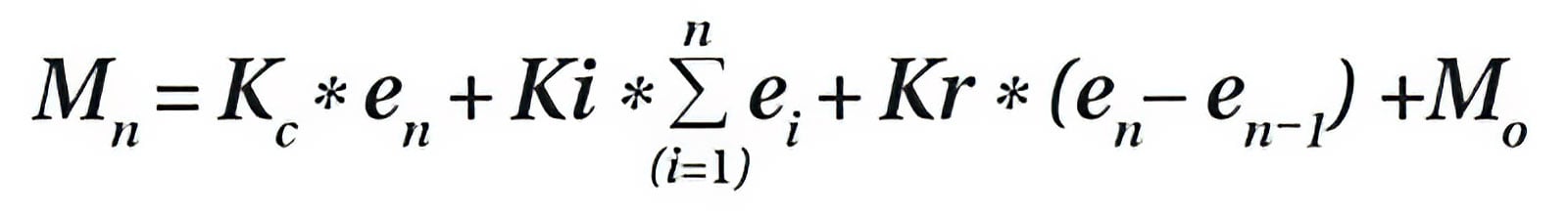
where:

M_n  is the control output at the moment of time n. This is the gain or response output, such as 0 -100%, sent to the controlled device.

e_n is the error at the moment of time n calculated by subtracting the desired set point from the actual process variable (SP - PV_n).

K_c  * e_n is the proportional term (P). K_c is the proportional gain coefficient and becomes fixed once the proper value is found during tuning.

Ki * ∑ ⁿ_i  =1 e_i is the integral term (I). This is the sum of the calculated errors from the first sample (i = 1) to the current moment n multiplied by Ki, the integral coefficient. Ki is calculated using the formula: Ki = K_c * sample rate/integral time.

Kr * (e_n − e_n−1) is the derivative term (D). It is the error now (e_n) minus the previous sample error (e_n−1), with the result multiplied by the derivative coefficient Kr, which is calculated using the formula: Kr = Kc * (derivative time/sample rate). The derivative term looks at the error now and the error before. It also determines how rapidly the error is increasing or decreasing, and adjusts the output as needed.

M_o is the control output initial value. It is also the value transferred if switching from manual to autoloop control.

A PI example

Applying this PID equation to a temperature control example shows how the P, I, and D terms work together. In this example, an oven is controlled to a desired temperature set point of 350°F (figure 1). As a starting point, the following parameters are used.

• Kr = 0 (This sets the derivative time to zero, making this a PI controller, which is a good starting point.)
• K_c = 3 (proportional gain)
• Ts = 60 second sample rate
• Ki = 1 (set integral time to 180 seconds as Ki = K_c * (sample rate/integral time) or Ki = 3*60/180 = 1
• M(0) = 30 (initial control output)

The graph (figure 2) charts temperature fluctuation over the past 9 minutes. The graph shows that the temperature is stable for the first five samples before dropping 20°F at sample six. The error at sample six is: e(6) = SP - PV = 350 - 330 = 20. The sum of all errors can also be calculated: ∑ e_i  = (e(1) + e(2) + e(3) + e(4) + e(5) + e(6)) = (0+0+0+0+0+20) = 20.

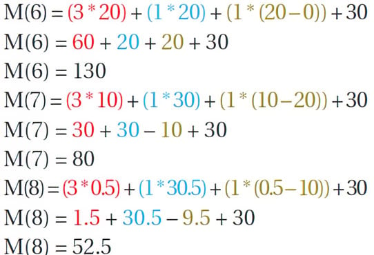
Combining the parameters and calculated values, the loop at sample six is solved as follows, where red is the proportional, blue is the integral, and green is the derivative term:

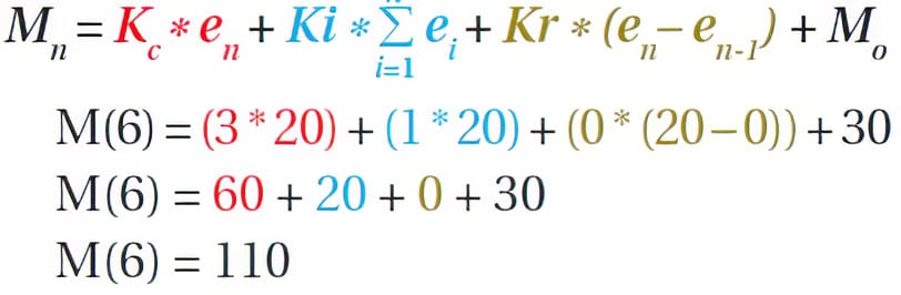
The result is 80 more than the initial control output of 30, with the proportional term providing most of the increase. The controller converts this result into an analog output to the controlled device-a heating element in this example-in the form of a 4-20 mA or 0-10 VDC signal.

As the control output drives the temperature toward the set point, at sample seven the error is decreasing, so e(7) = SP - PV = 350 - 340 = 10. At this time, the sum of all the sample errors is ∑  e_i = ((e(1) + e(2) + e(3) + e(4) + e(5) + e(6) + e(7)) = (0+0+0+0+0+20+10) = 30). At this moment in time, the result of the equation is:

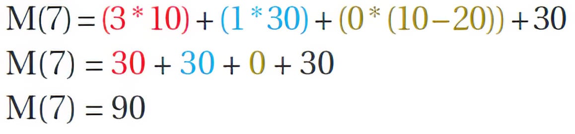
With the error corrected, the output decreases due to the drop in the proportional term, even though the integral term increased. At sample eight, the PV temperature recovers, to 349.5°F, making the sum of all errors 30.5. At this moment in time, the control output is:

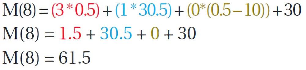
Now the proportional term is approaching zero, and the integral bias is having more effect on the control output. While the proportional term has decreased with the error from 60 to 30 to 1.5, the integral term has increased from 20 to 30 to 30.5. This highlights a loop tuning tip: with large error, the proportional term drives the output, and with small error, the integral term takes control.

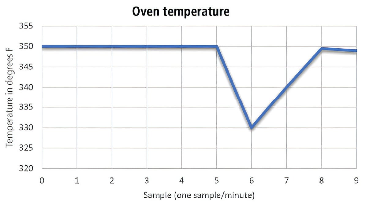Figure 2. This chart shows how the process variable changes in a PID temperature control application for an industrial oven.

Add a little D for stability

The derivative term adds stability to the control loop. When a rapid rate of change occurs, such as the 20°F drop at sample six, there is a risk of instability, which the derivative term reduces, while adding correction.

For example, if the derivative coefficient is changed to Kr = 1 by setting the derivative time (Td) to 20 seconds (Kr = Kc * (derivative time/sample rate) or Kr = 3*20/60 = 1), the control output at samples six, seven, and eight would become:

P, PI, then PID manual tuning

A process does not always require a three-mode PID control loop. Many applications run fine on only PI terms and some on just the P term, so it is common to disable parts of the PID equation. Selecting appropriate values for the gain (Kc), reset (Ti), and rate (Td) makes a P, PI, PD, I, ID, and D loop possible. This is also what is done to tune the PID loop manually.

It is difficult to tune all values of a PID control loop at once. To start, it is better to cancel out the integral and derivative, and tune the proportional term. Find a proportional value that provides a quick response of the process variable. Raise the proportional term until the PV becomes unstable and oscillates, and then reduce it until a stable response is achieved with slight oscillation or error. With a stable PV, add a small value for the integral term to help the error reach zero. The error will get smaller when this term is approaching the optimal value. At this point, the PI control should have the desired response with a stable PV and minimal error.

With many applications, especially temperature control, a PI loop is all that is needed. The derivative term is used in other applications, but it can slow the control response. It reduces gain when large rates of change in the PV are detected to reduce possible overshoot. This often causes undershoot-an over-dampened and slower response. Although each PID term can be manually entered to tune the control loop, the PID processing engine in some PLCs and advanced controllers can autotune the loop by automatically calculating the values.

Autotuning

Autotuning, if available in the controller, often reduces or eliminates the trial and error of manual PID tuning. In most cases, autotuning a control loop will provide terms close to optimal values. However, it is often necessary to perform some manual tuning to attain optimal values.

Many temperature controllers and PLCs provide an automatic tuning function (figure 3). During the autotune cycle, a controller controls the output value while measuring the rate of change, overshoot, and response time of the process. The Ziegler-Nichols method is then often used to calculate the controller PID term values.

Typically, the Ziegler-Nichols method creates a square wave on the control output to create a step response that is measured and analyzed. Based on the response of the PV, the autotune function calculates the terms and the sample time. Several full-span step cycles are used to compute the terms/gains.

When manually tuning a loop, take the time to understand the equation and start with the proportional term. With a responsive and stable PV, add the integral to the equation, and then add derivative if necessary. When an autotune function is used, a little adjustment to the terms may be all that is needed to optimize the control loop.

A version of this article also was published at InTech magazine.