

This guest blog post is part of a series on loop tuning. This blog post is Part 3 in the loop tuning series. Click these links to read Part 1 and Part 2.
The two most common categories of process responses in industrial manufacturing processes are self-regulating and integrating. A self-regulating process response to a step input change is characterized by a change of the process variable, which moves to and stabilizes (or self-regulates) at a new value. An integrating process response to a step input change is characterized by a change in the slope of the process variable. From the standpoint of a proportional, integral, derivative (PID) process controller, the output of the PID controller is an input to the process. The output of the process, the process variable (PV), is the input to the PID controller.
In Part 1 and Part 2 of this series, I presented tuning a PID controller for the basic “integrating” and “first-order, self-regulating” process responses. These responses are shown in figure 1. However, in some cases, the process response has more complex dynamics than those discussed in these two articles. The following complex process responses have been observed in the processes of many industries, including chemical, refining, petrochemical, pulp and paper, oil and gas, and pharmaceutical.
- self-regulating, second order, overdamped
- self-regulating, second order, underdamped
- self-regulating, second order plus lead
- self-regulating, second order plus lead with overshoot
- self-regulating, second order, nonminimum phase
- integrator plus first-order lag
- integrator plus first-order lead
- integrator plus nonminimum phase
The two most common of these complex dynamic responses are the “self-regulating, second-order, overdamped” and the “integrator plus first order lag” responses.
Another topic that is often overlooked when tuning PID controllers is the concept of resonance. When a PID controller is used on a process that has dead time (and all have some!), the closed-loop response has a resonant frequency at which it will amplify variability with frequency components at or near the resonant frequency. The more aggressive the tuning is, the higher the amplification.
This article covers the tuning of a PID controller for two of the most common complex dynamic responses—“self-regulating, second order, overdamped” and “integrator plus first order lag”—and the concept of resonance.
Challenges
It is rare to have a perfect model fit to an actual process response. Thus, the goal is to obtain a reasonably “good” model fit. This involves selecting a model type that is “complex” enough to be a good fit to the process response.
The two most common of the complex dynamics are the self-regulating, second-order, overdamped (hereinafter called “self-regulating second order”) and the integrator plus first order lag (hereinafter called “integrator plus lag”). Figure 1 contrasts the response of a self-regulating, first order to a self-regulating, second order and an integrator to an integrator plus lag.
The closed-loop response of a tuning method should be selectable in order to optimize the process performance that may or may not require optimized control loop performance. Optimizing the process performance may require that the loops in the unit have a coordinated response: either a very slow response to use process capacity to absorb variability or a very fast response to maximize regulation of load disturbances.
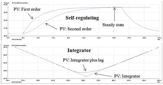 Figure 1. Comparison of a first-order to a second-order self-regulating response, and the comparison of an integrator to an integrator plus lag response
Tuning for a second-order, self-regulating process
A tuning methodology called lambda tuning addresses these challenges. The lambda tuning method allows the user to choose the closed-loop response time, called lambda, and calculate the corresponding tuning to achieve the desired response time. The lambda time is chosen to achieve the desired process goals and stability criteria. This could result in choosing a small lambda for good load regulation, a large lambda to minimize changes in the controller output and manipulated variable by allowing the PV to deviate from the set point, or somewhere in between these two extremes. More importantly, the lambda of the loop can be used to coordinate the responses of many loops to reduce interaction and variability.
Lambda tuning for self-regulating processes can cause a closed-loop response that is slower or faster than the open-loop response time of the process. Though lambda is defined as the closed-loop time constant of the process response to a step change of the controller set point, the load regulation capability is also a function of the lambda of the loop. The response to a step set point change and a step load change for a self-regulating process response with lambda tuning is shown in figure 2.
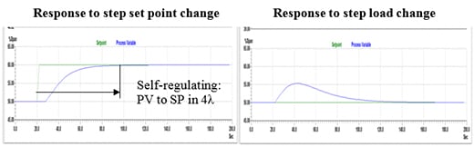 Figure 2. Response of lambda tuning for a self-regulating process for a step set point and a step load step change
Self-regulating process responses typically include dead time and can usually be approximated by a “first-order plus dead time” or “second-order plus dead time, overdamped” response. This article describes the lambda tuning procedure when the process response can be best approximated by the latter. The lambda tuning for a second-order plus dead time response can be approximated with manual analysis and calculations. A more rigorous analysis is required for more exact tuning.
Procedure
The lambda tuning method for self-regulating processes has three steps:
- Identify the process dynamics.
- Choose the desired closed-loop speed of response, lambda.
- Calculate the required PID tuning constants.
Figure 3 shows the dynamic parameters of a self-regulating, second-order process, which include dead time (Td), in units of time; primary time constant (tau 1), in units of time; secondary time constant (tau 2), in units of time; and the process gain (Kp), in units of percent controller PV/percent controller output. Typically several step tests are performed; the results are reviewed for consistency; and the average process dynamics are calculated and used for the tuning parameter calculations. If the controller output goes directly to a control valve, any significant dead band in the valve will reduce process gain if the output step was a reversal in direction. If the controller output cascades to the set point of a “slave” loop, the slave loop should be tuned first.
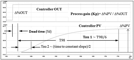 Figure 3. Step response showing the process dynamics of a second-order, overdamped self-regulating process, which include dead time, primary time constant, secondary time constant and process gain. T98 is the time required for the process to reach 98 percent of its final change.
The next step is to choose the lambda to achieve the desired process control goal for the loop within the allowable stability margin for the expected changes in process dynamics. A shorter lambda produces more aggressive tuning with less stability margin. More aggressive tuning also has a larger amplification of disturbances with a period of oscillation near the resonant period of the loop. A longer lambda produces less aggressive tuning and more stability margin. It is not uncommon for the process dynamics, particularly the process gain, to vary by a factor of 0.5 to 2. If testing during different conditions reveals that the process dynamics change significantly, then an additional margin of stability is required. The process response could also be “linearized,” or adaptive tuning could be used.
If the potential change in process dynamics is unknown, starting with lambda equal to three times the larger of the dead time or time constant provides stability even if the dead time doubles and the process gain doubles. If it is desirable to coordinate the response of loops to avoid significant interaction, the lambda of the interacting loops can be chosen to differ by a factor of five or more. For cascade loops, the lambda can be chosen to ensure the slave loop of the cascade pair has a lambda 1/5 or less of the master control loop.
This blog post is Part 3 in the loop tuning series. Click these links to read Part 1 and Part 2.
If derivative is used, the lowest recommended lambda for a self-regulating, second-order process is approximately equal to the larger of the dead time or lag time constant. If derivative is not used, then the minimum lambda varies depending on the amount of the secondary time constant, but is in the range of two times (dead time + tau 2). Both of these lower limits on lambda result in aggressive tuning with a very low gain and phase margin. Thus, moderate increases in the dead time or process gain can cause instability of the loop. Using properly set derivative action actually provides more stability for these complex dynamics.
From a stability standpoint, there is no upper limit on the lambda. If the lambda is not chosen based on a coordinated response, a good starting point for stability for PI or PID tuning is:
Equation 1. Lambda = 3 × (larger of dead time or time constant)
The tuning performance can be monitored for a time period and adjusted to be a shorter or longer lambda as needed.
The final step is to calculate the tuning parameters from the process dynamics. Care should be taken to use consistent units of time for the dead time and the lambda. For a self-regulating, second-order process response, the controller gain, integral time, and derivative time are calculated with the following equations. These equations are valid for the series (sometimes called classical or interactive) form of the PID implementation. Note that only the controller gain changes as lambda (λ) changes. The integral time remains equal to the time constant regardless of the lambda chosen. Conversion of the tuning from series PID form to standard form (sometimes called ideal, noninteractive) is provided in the last section.
Equation 2. Integral time = Primary time constant (tau 1)
Equation 3. Controller gain = 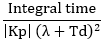
Equation 4. Derivative time = Secondary time constant (tau 2)
Example
Consider the simulated temperature controller shown in figure 4. The temperature controller, TIC-302, manipulates a properly selected control valve that has a high-performance digital positioner.
Figure 5 shows a step test of the temperature controller to identify the process dynamics. Several such steps were analyzed, and the average process dynamics were calculated. The process gain is 1.0%PV/%OUT; the dead time is 20 seconds; the primary time constant is 80 seconds; and the secondary time constant is 60 seconds.
In this example, there are no “loop response coordination” requirements, so the initial lambda is chosen to be 3 × (larger of dead time or primary time constant) = 3×80 seconds = 240 seconds.
Now, the tuning for a series PID form can be calculated with the lambda tuning rules.
Integral time = Primary time constant (tau 1) = 80 seconds
Controller gain = .png?width=104&name=Equation%203%20(1).png) = 80 seconds/((1.0) × (240 sec + 20 sec)) = 0.31
= 80 seconds/((1.0) × (240 sec + 20 sec)) = 0.31
Derivative time = Secondary time constant (tau 2) = 60 seconds
If the process dynamics have been tested or proven over time to be consistent in the overall operating range, more aggressive tuning may be desirable. The following table shows the tuning for different values of lambda. Note that the integral and derivative time remains the same for all choices of lambda.
| Lambda (seconds) | Gain | Integral time (seconds) | Derivative time (seconds) | Amplitude ratio |
| 240 | 0.31 | 80 | 60 | 1.09 |
| 120 | 0.57 | 80 | 60 | 1.12 |
| 80 | 0.8 | 80 | 60 | |
| 20 (minimum value = dead time) | 2.0 | 80 | 60 |
Figure 6 shows the response to a step set point and a step load change for each of the lambda values in the table. Note that the tuning is stable for shorter lambda values than the starting point of 3 × (larger of dead time or time constant). However, this is with unchanging process dynamics in a simulator. Additional tests on a real process, in different operating conditions, will help determine how consistent the process dynamics are and whether more aggressive tuning is stable and provides the desired process performance.
The next step is to choose the lambda to achieve the desired process control goal for the loop within the allowable stability margin for the expected changes in process dynamics. The same warnings about variations in process dynamics, control valve performance issues, and the need to tune the slave loop first in a cascade arrangement apply to this process response. Without using derivative, the minimum lambda considering stability and resonance requirements is approximately 3 × (dead time plus lag time constant). Using derivative, the minimum lambda considering stability and resonance requirements is approximately the larger of the dead time or the lag time constant. If a lambda is chosen that is near these limits, the resulting tuning should be tested on a simulator to verify its stability and resonance. Analysis tools can provide a more accurate calculation of lambda tuning values and the limits of lambda based on stability and resonance.
The final step is to calculate the tuning parameters from the lambda and process dynamics. Care should be taken to use consistent units of time for the dead time, lag time constant, and the lambda. For an integrator plus first-order lag process response, the controller gain, integral, and derivative times are calculated with the following equations. These equations are valid for the series (sometimes called classical, interactive) form of the PID implementation. Note that both the PID gain and integral time change as lambda changes. The derivative time remains the same for all choices of lambda. Conversion of the tuning from series PID form to a standard form (sometimes called ideal or noninteractive) is provided in the last section.
Equation 5. Integral time = 
Equation 6. Controller gain = .png?width=104&name=Equation%203%20(2).png)
Equation 7. Derivative time = Lag time constant
Example
The process shown in figure 8 will be used as an example. The level controller, LIC-102, manipulates a properly tuned flow controller, FIC-102. The level process on these types of applications typically has an integrator plus lag response.
Figure 9 shows a step test of the level controller, LIC-102, to identify the process dynamics. Several such steps were analyzed, and the average process dynamics were calculated. The process gain is 0.005%PV/second/%OUT; the dead time is 20 seconds; the first-order lag time constant is 60 seconds.
The next step is to choose the lambda. One method to choose the lambda is the “allowable percent PV deviation” method. If it is desired to keep the %PV within an “allowable deviation” (AD) from its previous value due to step change load disturbance (MLD, in units of the %OUT of the controller), then the required lambda can be calculated from equation below.
Equation 8. 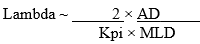
For this example, AD = 20%PV, MLD = 50%OUT. From above, Kpi = 0.005 %PV/sec/%OUT.
Thus, Lambda = (2 × 20%PV)/(0.005%PV/sec/%OUT × 50%OUT) = 160 seconds.
Now, the tuning for a series PID form can be calculated using equations 5–7.
Integral time = = 2 × 160 seconds + 20 seconds = 340 seconds
Controller gain == (340 sec)/((0.005 %PV/sec/%OUT) × (160 sec+20 sec)2)
= 2.1
Derivative time = Lag time constant = 60 seconds
The following table shows the tuning for several different values of lambda. Note that both the PID gain and integral time change as lambda changes. The derivative time remains the same for all choices of lambda.
| Lambda (seconds) | Gain | Integral time (seconds) | Derivative time (seconds) |
| 240 | 1.48 | 500 | 60 |
| 160 | 2.1 | 340 | 60 |
| 60 (minimum value ~ larger of lag or dead time) | 4.4 | 140 | 60 |
Figure 10 shows the response to a step set point and a step load change for each of the lambda values in the table. Note that the tuning is stable for much shorter lambda values than the starting point of 3 × (larger of dead time or time constant). However, this is with constant process dynamics in a simulator. Additional tests on a real process, at different operating conditions, will help determine how consistent the process dynamics are.
Meeting process goals
Most published PID controller tuning methods are designed for optimum loop performance, not necessarily optimum process performance. Optimizing the process performance may require that the loops in the unit have a coordinated response, a very slow response to utilize process capacity to absorb variability, or a very fast response to maximize regulation of load disturbances. The lambda tuning method provides the ability to tune the PID controllers in a process system to achieve process performance goals regardless of the loop requirements. The lambda tuning method can be used for all of the common complex dynamics that were listed in the introduction.
Loop resonance and variability amplification
The combination of a PID controller (with P, PI, or PID tuning) is used on a process that has dead time; the closed-loop response will have resonant frequency at which it will amplify variability with frequency components at or near the resonant frequency. And, the more aggressive the tuning is, the higher the amplification. Figure 11 shows a frequency response plot (Bode plot) of a PV disturbance for the temperature loop, TIC-301, used in the example for a self-regulating, second-order process response. The aggressive tuning of lambda = dead time = 20 seconds results in an 82 percent amplification of any variability with a period near 138 seconds. In other words, if there is variability that has a period near 138 seconds with the controller in manual, putting the controller in automatic will increase the variability by 82 percent! Interestingly the limit cycle from a poorly performing control valve might have a period around this value! Figure 12 shows a time series presentation of the data to illustrate this concept. Figure 13 shows how the aggressiveness of the tuning affects the amplification ratio. The concept of resonance and variability amplification should be considered in the controller tuning process.
Conversion of the tuning from to series PID form to a standard form
Equations 9–11 below can be used to convert tuning from a series PID form to a standard PID form. The equations are based on series PID tuning parameters with the following units.
- controller gain: %OUT/%PV (often said to have “no units”)
- integral time: seconds
- derivative time: seconds
Equation 9. Standard PID gain = Gain × (integral time + derivative time)/(integral time)
Equation 10. Standard PID integral time = (integral time + derivative time)
Equation 11. Standard PID derivative time = (integral time × derivative time)/(integral time + derivative time)
Useful models
It has been said that “All process models are wrong, but some are useful.” Of the more than 4,000 process responses that I have analyzed in the past 15 years, I have never measured the same exact model parameters for different tests of the same process! Thus, the goal for process model–based tuning is to identify a reasonable fit to a particular process model. The better the model fit, the more accurate the tuning and results will be. In some cases, this requires choosing a more complex process model. The consistency (linearity) of the process response will affect the margin of stability that is required when tuning the loop. In some cases, techniques to linearize the process response from the perspective of the controller may be required. During the controller tuning process, the process objectives should considered when choosing the control loop objective. Once the control loop objective is identified, a tuning methodology that can achieve the desired control loop object will help achieve the process objectives.
A version of this article also was published at InTech magazine.

