The following discussion is part of an occasional series, "Ask the Automation Pros," authored by Greg McMillan, industry consultant, author of numerous process control books, and 2010 ISA Life Achievement Award recipient. Program administrators will collect submitted questions and solicits responses from automation professionals. Past Q&A videos are available on the ISA YouTube channel. View the playlist here. You can read all posts from this series here.
Looking for additional career guidance, or to offer support to those new to automation? Sign up for the ISA Mentor Program.
Mathew Howard, Area Process Systems Engineer for Sappi North America, has posed very detailed and practical questions on process control, as has been seen in the Mentor Q&A post, “What Are Some Ways to Improve and Prioritize Feedforward and Fast Feedback Control?” He has also provided his perspective in the Mentor Q&A, “What Can be Done to Increase Innovation in PID Control?”
He has expressed the following concerns:
“My mill is going through a huge turnover of knowledge due to the retirement wave being the same age as major parts of the mill. I have also found that many controls and systems folks were hired in the late 80s and mid 90s when the DCS systems were being installed. This has culminated in a huge loss of expertise, even with the suppliers.
Jacques Smuts puts it well in the forward to his book on how the young control engineer is being pushed to focus on management and APC applications. ‘The harvest is plentiful, but the laborers are few.’ I like math, Chem E, and the business too much to ignore the base controls. I am thankful that the old guys care enough to pass on their knowledge. I wish there were a few more of us young guys interested and supported by our companies.”
Mathew Howard’s Question
What can be done to control a process variable that is being measured by an instrument with slow, periodic updates to the signal? What can be done to smooth out the signal with a “soft sensor” or “virtual instrument?” If this is not possible, what are the limitations of traditional PID control?
Russ Rhinehart’s Answer
Consider a cascade structure. Find an intermediate variable in the process (some variable between the manipulated variable and the analyzer) that is both easily measured and provides an early indication of what the analyzer will eventually indicate. Have a set point for the intermediate variable and use the current manipulated variable to control the intermediate variable, not the delayed analysis value. Then, use feedback control to adjust the intermediate variable set point to keep the analysis value at its set point.
This traditional cascade structure is common in distillation. Tray temperature is the intermediate variable, and feedback from a downstream delayed composition analysis is used to adjust the tray setpoint. Sometimes this intermediate set point is adjusted in response to other variables, such as column pressure.
If the delayed analyzer measurement is noisy (subject to any number of types of random fluctuations), then after each sampling, noise will shift the intermediate setpoint, making the process adjust to the analyzer noise. In 6-sigma and Statistical Process Control terminology this is tampering.
Search for W. Edwards Deming’s funnel experiment. You could use a first-order filter to temper the composition analyzer noise, but with either large deadtime or end-of-batch measurements, I think this introduces a significant undesirable lag. I’d recommend a statistical CUSUM filter which holds an average value, and only changes it when there is statistically adequate justification.
Greg McMillan’s Answer
Inferential measurements can definitely fill in the blanks if they include all the dynamics in the process’s response. The identification of the dynamics (e.g., total dead time, primary and secondary time constants, and open loop gain) and how they change with operating conditions is essential.
For example, the process gain and process dead time are often inversely proportional to feed rate and thus production rate and all of the loop dynamics are affected by automation system dynamics, most notably those in the final control element and the measurement. This is quite challenging because methods of providing inferential measurements by collection of plant data, such as neutral networks and projection to latent structures (partial least squares), do not have the spectrum of operating conditions or changes in manipulated variables needed; consider the transfer of variability from the controlled variable to the controller output required to identify an accurate dynamic response needed for an inferential measurement. They may use a dead time but rarely time constants to match the process dynamics. However, they can uncover unforeseen relationships useful in developing and improving experimental and first principle models.
Data from changes in controller setpoints over the entire operating region is needed. Loop tuning software can be setup to identify all the dynamics, including the dead time from slow signal updates of discrete devices and analyzers. The dead time from slow updates is ½ the update time interval plus the entire latency, which can be quite large for wireless communication. For negligible latency, the deadtime is simply ½ the update time and is extremely large for analyzers where the dead time is typically 1.5 times the cycle time, since the latency is the cycle time because of the analysis being done at end of the cycle time.
There may also be sample transportation delays for analyzers. The advantage offered by the inferential measurement is the omission of these measurement delays. There can be synergy from experiments done in a digital twin with an adapted first principle model to provide more information on process gains, time constants, and interactions as a result of changes in production rate and operating conditions.
The Control Talk article, “Bioreactor control breakthroughs: Biopharma industry turns to advanced measurements, simulation and modeling,” shows how a digital twin first principle model can be non-intrusively adapted online to provide inferential measurements of cell growth rate and product formal rate. First principle models tend not to have as much dead time, noise, or limit cycles seen in actual processes. Special care must be taken to include final control element deadband and resolution limits, heat transfer and measurement lags, and transportation and mixing delays.
Simple tests in the plant can provide information on noise and dead time that needs to be added to the model. Regardless of the type of inferential measurement, it must be periodically corrected by an actual process measurement or analyzer result typically by a bias correction that is simply slightly less than ½ (e.g., 40%) of the difference between the inferential measurement synchronized with the actual measurement with outliers omitted and noise reduced per Russ Rhinehart’s answer.
It is important to realize that the inferential measurement used for control benefits may not have the measurement dynamics, but measurement dynamics must be included for synchronization with the actual online measurement for periodic correction. For example, a simple synchronization would involve passing the inferential measurement through filters corresponding to sensor lags and a dead time block to account for transportation delay and update rate and latency. For off-line (e.g., lab) analyzers, the sample must be time-stamped and the inferential measurement from historian data at the time the sample was taken is compared to the subsequent off-line analyzer result for correction. A limit switch on the sample valve or the beginning of a jump in measurement by a bare thermocouple element or conductivity probe in the sample volume can be used to timestamp the sample. If coating or solids are a potential issue, the sample volume needs to be flushed after the sample is removed from the holder.
A simple physics-based model using material and energy balances can be used to provide the process gain and process time constant. In the Control Talk article, “Optimizing process control education and application,” John Hedengren, who leads the Process Research and Intelligent Systems Modeling (PRISM) group at Brigham Young University (BYU), offered the following example:
“A few years ago, we were switching the method to regulate the pressure of a gas-phase polymer reactor. We fixed the catalyst poison flow (old controller output) and performed a step test on the fluidized-bed level (new controller output) to get the pressure response. The pressure moved in the opposite direction to the expected response. The multi-hour step test failed to give us the data needed for the initial PID controller because of a disturbance that occurred during the test.
We turned to a simplified physics-based model to give us an approximate time constant and gain. This gave us confidence to repeat the step test. This time, the expected and measured results matched, and we implemented the new control scheme with substantial benefits to the company.”
First principle models using a simple charge balance that includes the effects of carbon dioxide absorption and conjugate salts can provide the titration curves needed to quantify the extreme pH nonlinear gain that is often a mystery. This is the key to equipment and automation system design besides offering an inferential measurement.
If an inferential measurement is too difficult due to unknowns, the PID algorithm may offer options to deal with the disruptions from slow updates. One simple option is to time the execution of the PID to coincide with the update. Another more powerful method is the enhanced PID described in Annex E of the ISA 5.9 Technical Report on PID Algorithms and Performance that uses external-reset feedback to give a more intelligent integral and derivative action (taking into account the time between updates) plus protection against valve and measurement failures.
Furthermore, the enhanced PID eliminates the need for retuning if the time between updates increases and the tuning simplifies to a PID gain being the inverse of the open loop gain if the update time is larger than the 63% process response time for self-regulating processes. Strangely enough, this can be used with incredibly large and variable delays from at-line and lab analyzer results. The additional dead time from slow updates does make the PID more vulnerable to unmeasured load disturbances, but the setpoint response is just limited by process dynamics (not measurement dynamics) and tuning. In the ideal case where the PID gain is exactly equal to the inverse of the open loop gain, just a single change in output at the time of the setpoint change can result in the desired process response greatly reducing rise time, overshoot, and settling time. While the original intent was to improve control with wireless devices, the greater impact is improving control with at-line and offline analyzers.
For more on the enhanced PID, see the following white paper, “PID Enhancements for Wireless.”
Mark Darby’s Answer
The typical situation where the signal update is slow is because of the control of a stream composition or property. The measurement may be an online analyzer, or a lab measurement of a sample periodically collected from the process. An analyzer sampling time may vary from a few minutes to 30 minutes or longer if the analyzer is connected to multiple streams. The sampling interval for lab measurements may vary from as frequently as a few times per day, to as slow as weekly or possibly even slower.
When it is desired to control with a slow update, an obvious candidate is an inferential (aka soft sensor), which predicts the composition or property using continuously measured values (temperature, pressure, etc.). Even when the signal updates are relatively fast, a soft sensor may make sense if the analyzer or sampling system is unreliable (for example, a difficult service due to plugging or contamination). Another advantage is that validity checks are easily incorporated and performed before a model update. Checks can include rate of change, min/max, and statistical checks (like Russ’s recommendation above), which allow an update only when a measurement change is significant relative to the noise. In addition, model update parameters are often filtered (i.e., only a fraction of the change is implemented); however, note that this filtering is only applied when a new measurement occurs.
Before deciding to develop an inferential, it is first worthwhile to consider if an existing analyzer can be used. For example, can an existing multi-stream analyzer be modified to perform more frequent analyses at the expense of a slower frequency of lesser important streams, or can an existing analyzer be made more reliable by modifying certain parts, improving the sample system, or proving more frequent maintenance? If an analyzer is not available, it could be worth investigating a new analyzer, for example a spectrum analyzer, which is based on wavelengths that are fit to the composition or property of interest.
A starting point for the development of a soft sensor is historical data. The only caveat is that excessive data compression techniques must not be used. The best situation is when the desired composition or property measurement can be predicted from temperature(s) and pressure(s), and not solely from flow measurements; for example, predicting a distillation column product composition from a pressure compensated temperature instead of a reflux flow. Historical data for this case is often preferred to manipulated variable (MV) testing as it will pick up the effects of unmeasured disturbances and, thus, more nearly reflect the situation the model will face when put online. If a predictive temperature measurement is not available, it is worth investigating if one can be installed or an existing measurement has moved to another location.
Simulation—either steady-state or dynamic—can guide the decision. If temperature(s) cannot be found, one is left modeling with flows or flow ratios (which can be better since it is an intensive variable), but this will be inferior as there is no mechanism for picking up unmeasured disturbances, except by feedback of the actual measurement. It may be necessary to consider multiple flows if their effect is significant. It may be necessary in this situation to use simulation data to develop the form of the model and to generate data for the model.
There are additional issues with lab data. When modeling, it is important to have an accurate timestamp to time align the lab values with the model inputs. Once a model is put online, it is similarly necessary for performing a model update to know when a lab sample was collected (from the process, not when it was analyzed in the lab) to, again, align with the lab measurement when it is reported. If an automatic detection method is not implemented (by one of Greg’s approaches mentioned above), a manual approach must be used. A typical approach is for the operator to manually set a digital switch on a display in the DCS when notified when a process sample is taken. This action then triggers a timestamp collection, or it forces the corresponding model measurements to be saved for later model update when the lab sample is reported.
There is more than one way to update the model. Here’s how I look at the problem:
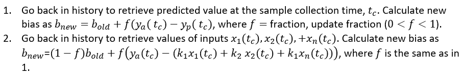
Consider the case where a soft sensor is developed by fitting a static model and assume the model is of the following (linear) form:
 Options for updating:
 A few words on the regression technique used to fit a soft sensor. It can be linear or nonlinear, static, or dynamic. With online analyzers, a dynamic model is often used. With lab data, a static model is often used. In the case of a static model, it is often required to filter or average the model inputs to remove undesirable affects in the soft sensor, such as jumps or inverse response. Care should be taken to not overdo it, thereby adding unnecessary lag.
Since process data is often highly correlated, one needs to be careful when developing a multi-input model. Iteration on the selected inputs by introducing new input variables step wise into the regression can be used to avoid ill-condition leading to a poor model. Alternatively, as Greg mentioned above, partial least squares (PLS) can be used, which avoids the correlation problem.
The same problem exists with neural net modeling. Some types of networks handle this automatically, at least to a degree. An approach that has been used with neural nets is to preprocess the inputs using principle component analysis (PCA) (iterating on the number of principle components) and to feed these new variables to the neural net. In my opinion, the correlation issue has not been addressed sufficiently for process applications with neural nets. Also, engineering knowledge can guide variable selection as well as the use of calculated variables as model inputs.